In this article, we will be building a dummy AI model that learns the temperature conversion formular from data values generated using the actual formular.

The code can be found on github

Motivation for building this dummy model:

To Show how a model can be built and evaluated using the keras framework

Background

The temperature conversion formular from Degrees Fahrenheit to Degrees Centigrade is given below in python:

  centigrade = (fahrenheit - 32)*(5/9)

Given some data values generated using the above formular, we want to train a simple AI model to learn the formular and be able to predict temperature in Centigrade given unseen values of temperature in Fahrenheit.

Implementation in Python and Kera

We shall begin by importing the necessary python modules

1
2
3
4
5
6
7
8
9
10
11
12
13
14
"""
A dummy AI model for predicting temperature in degrees centigrade
given degrees fahrenheit 
"""

#
#import necessary modules
#
from sklearn.model_selection import train_test_split
from keras import models
from keras import layers

import numpy as np
import matplotlib.pyplot as plt

We then go ahead to generate a dummy dataset using the temperature conversion formular

1
2
3
4
5
6
7
8
9
10
11
12
13
14
#
# create  a dummy dataset
#
#centigrade = (fahrenheit - 32)*(5/9) # conversion formula
sample_size = 1000
test_size = 0.25

# train set
x_train = np.random.uniform(1,100,(int(sample_size*(1-test_size)),1)) # generate random Fahrenheit values between 1 and 100
y_train = np.array([(fahrenheit - 32)*(5/9) for fahrenheit in x_train]) # calculate corresponding Centigrade values

# test set
x_test = np.random.uniform(101,200,(int(sample_size*test_size),1)) # generate random Fahrenheit values between 101 and 200
y_test = np.array([(fahrenheit - 32)*(5/9) for fahrenheit in x_test]) # calculate corresponding Centigrade values

Note how we specify different value ranges for the train and test set using the uniform function in the random package of numpy, what the parameters mean is shown below:

np.random.uniform(lower value, higher value, size) 

The different ranges are specified so as to ensure we don’t leak test values into the train data set.

We go ahead to build the model, specifying the layers and the number of units :

1
2
3
4
5
6
7
8
9
10
11
12
13
14
#
# build the model
#
def build_model():
    """
    build a sequential dense neural network
    """
    model = models.Sequential()
    model.add(layers.Dense(64, activation='relu',
                           input_shape=(1,)))
    model.add(layers.Dense(64, activation='relu'))
    model.add(layers.Dense(1))
    model.compile(optimizer='rmsprop', loss='mse', metrics=['mae'])
    return model

Explanation of the model

The model is made of 3 densely connected neural network layers stacked together sequentially. The number of units in the first two layers has been chosen out of try and error, the stop condition being until when satisfying results are achieved. The last layer has only one unit since we expect the network to predict a single value. These units in the first two layers can be tweaked more to achieve better results.

During model compilation, the chosen loss function is mean squared error(MSE) since we want to minimize the difference between the model prediction and the actual expected values. We also chose to monitor the mean absolute error in the metrics, to see how much the model prediction diverges from the expected values.

After building the model, we go ahead to fit the training data onto the built model.

1
2
3
4
5
6
7
8
9
10
11
12
#
# model training
#
num_epochs = 20
model = build_model()
history = model.fit(x_train, y_train,
                        epochs=num_epochs, batch_size=8, verbose=1)
loss_values = history.history['loss']

mae_values = history.history['mae']

epochs = range(1, len(loss_values)+1)

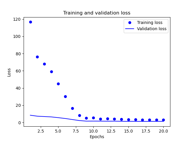
We chose to train the model for 20 epochs and a batch size of 8. Using pyplot from matplotlib, we can visualize the training process as below.

1
2
3
4
5
6
7
8
9
# training visualization
plt.figure()
plt.plot(epochs, loss_values, 'bo', label='Training loss')
plt.plot(epochs, mae_values, 'b', label='Validation loss')
plt.title('Training and validation loss')
plt.xlabel('Epochs')
plt.ylabel('Loss')
plt.legend()    
plt.show()   

We also go ahead to evaluate the model on the test data set, the results obtained are shown below:

1
2
3
4
5
#
# model evaluation
#
eval_mse, eval_mae = model.evaluate(x_test, y_test, verbose=1)
print("MSE=%s, MAE=%s" % (eval_mse, eval_mae))

[MSE=53.75002670288086, MAE=6.751595497131348]

The Results from the training process show that the model has learnt to fit the input values to the output values by around the 10th epoch. Further training maintains the loss and the mean absoulte error values almost constant. At this point, we shall make a decision of stopping the training at the 10th epoch so as to improve the model generalization on unseen data. The results of the evaulation, taking MAE as the bench mark, imply that we are off by almost 7 degrees centigrade which is quite large in actual sense.

Training the model again with an epoch count of 10, the new results from the model evalaution are shown below:

[MSE=18.294105529785156, MAE=4.252650260925293]

The above results show that the model has improved abit from the first MAE by about 2.5 degrees centigrade.

Let us go ahead to generate new data values in an unseen range so as to see how well the model performs on unseen data.

1
2
3
4
5
6
7
8
9
10
11
12
13
14
15
#
# application of the trained model, predicting values
#
x_new = np.random.uniform(201,500,(50,1)) # generate random Fahrenheit values between 201 and 500
y_new = np.array([(fahrenheit - 32)*(5/9) for fahrenheit in x_new]) # calculate corresponding Centigrade values

y_new_predicted = model.predict(x_new)
# plot predicted and actual
plt.figure()
plt.plot(y_new_predicted, 'b', label='Predicted Values')
plt.plot(y_new, 'g', label='Actual Values')
# plt.plot(y_new_predicted, y_new, 'b', label='Predicted Values')
plt.title('Predicted and Actual Values')
plt.legend()
plt.show()

The results of the plot of predicted values and the expected values are shown below:

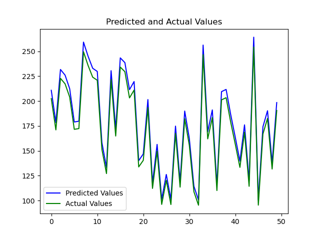
The results in the plot above show that the model has been able to learn the temperature conversion formular to some extent, the model is able to predict centigrade values with an average absolute error of about 4.2 degrees centigrade.

Improvement

Exposing the model to more data values and adjusting the number of layers and input units can help to improve on how well the model performs in predicting the values of the temperature conversion formular. Normalizing the temperature values before feeding them into the model could be another way of improving the performance.